Reinforcing Jack's Car Rental

Python is an excellent multipurpose language that I truly enjoy using for work and fun. For me probably shortened the development time by about 10 - 20 times compared to C++, all things being equal. This extraordinary convenience does not come for free, as the code speed suffers greatly when the hard lifting cannot be efficiently outsourced to a library like numpy. Going deeper into a Reinforcement Learning rabbit hole, I decided to check out Julia as a potential goldilock option. With this in mind, here is my take on a Q-Learning solution to “Jack’s Car Rental” problem that I have explored earlier.

To start, here is the text of the problem:

Jack manages two locations for a nationwide car rental company. Each day, some number of customers arrive at each location to rent cars. If Jack has a car available, he rents it out and is credited 10 by the national company. If he is out of cars at that location, then the business is lost. Cars become available for renting the day after they are returned. To help ensure that cars are available where they are needed, Jack can move them between the two locations overnight, at a cost of 2 per car moved. We assume that the number of cars requested and returned at each location are Poisson random variables, meaning that the probability that the number $n$ is $\lambda^ne^{-\lambda}/n!$ , where $\lambda$ is the expected number. Suppose $\lambda$ is 3 and 4 for rental requests at the first and second locations and 3 and 2 for returns. To simplify the problem slightly, we assume that there can be no more than 20 cars at each location (any additional cars are returned to the nationwide company, and thus disappear from the problem) and a maximum of five cars can be moved from one location to the other in one night. We take the discount rate to be $\gamma$ = 0.9 and formulate this as a continuing finite MDP, where the time steps are days, the state is the number of cars at each location at the end of the day, and the actions are the net numbers of cars moved between the two locations overnight.

As before, I seek to solve a Control problem and to determine the optimal policy $\pi(a | s)$ - the number of cars $a$ to be transferred from location 2 to location 1 (or vise versa) in order to maximise the expected value

$$\upsilon(S) = E_{\pi}(\sum_{t=1}^{\infty}\gamma^t R_t | S).$$

where state $S = (N_1, N_2)$ is given by the number of cars at the first ($N_1$) and second ($N_2$) locations. In mathematical terms, discount rate $\gamma$ = 0.9 means that 1 Dollar tomorrow is worth 90c today, the same 1 Dollar in 2 days is worth 81c today and so on.

Q-Learning

Being a probabilistic function, optimal policy $\pi(A | S)$ should return 1 if $A$ equals to the best number of cars $A^*$ to be moved between car parks and 0 for all other car values.

At the start of the next day, the number of cars at each location will be $AS =(N_1 - A, N_2 + A)$, which are called after-states (states that we find outselves in after taking an action). The reward for the next day depends on this after-state as well as the action taken, since it costs 2 Dollars to move one car between locations. With this in mind, optimal value can be written as

$$\upsilon(S_t) = \arg\max_A Q(S_t, A) = \arg\max_A E(\sum_{k=t+1}^{\infty}\gamma^{k - t} R_k | S_t, A) $$

Using the above expression and action-value $Q(S, A)$ for every state $S$ and action $A$ available in that state enable to determine the optimal value for that state as well as the optimal policy. Q-Learning constructs a set of successive approxamations to action-value $Q_1(S_t, A_t)\rightarrow Q_2(S_t, A_t) \rightarrow … \rightarrow Q_N(S_t, A_t)\approx Q(S_t, A_t)$ by using the following action-value update

$$Q_{t+1}(S_t, A_t) = Q_t(S_t, A_t) + \alpha(G - Q_t(S_t, A_t))$$

$$G = R_{t+1} + Q_t(S_{t+1}, A_{t+1}^*)$$

where $A_{t+1}^*$ is the optimal action according to the latest available estimate of the optimal policy $\pi_t(A | S_{t+1})$. After the above update step, optimal policy is recalculated.

As number of cars at the start of next day, along with the action, the reward can be symbolically written as $R_{t+1} = R_{t+1}(N_1 - A_t, N_2 + A_t, A_t) = R_{t+1}(AS_t, A_t)$. This indicates that the action-value update formula can be written in terms of action-states

$$Q_{t+1}(AS_t, A_t) = Q_t(AS_t, A_t) + \alpha(G - Q_t(AS_t, A_t))$$

Environment Setup

Armed with the above mathematical expressions, lets get to Julia implementation.

Here is a list of paramets from the problem’s text:

N_MAX_CARS = 20
A_MAX = 5
LAMBDA = [3, 4]
MU = [3, 2]
GAMMA = 0.9
R_A = -2
R_X = 10

Firstly, the envorinment that simulates car rental interaction with the customers renting and returning cars has to be set up. For this purpose it is convenient to pre-calculate possible numbers of rented X1, X2 and returned Y1, Y2 cars and their respective probabilities (same names with a prefix “p”). Even though in reality there is an potentially infinite number of returned or requested cars, it can be truncated at some reasonably low probability value. I opted for cutoff of 8 times the mean value. The Environment function looks like this:

function Environment(S::State, A::Int64)
    """
    Evaluate new state and reward
    """
    new_S = State(S.N1 - A, S.N2 + A)
    
    x1 = min(sample(X1, Weights(pX1)), new_S.N1)
    x2 = min(sample(X2, Weights(pX2)), new_S.N2)

    reward = R_X*(x1 + x2) + abs(A)*R_A
    new_S.N1 -= x1
    new_S.N2 -= x2
    
    y1 = min(sample(Y1, Weights(pY1)), N_MAX_CARS - new_S.N1)
    y2 = min(sample(Y2, Weights(pY2)), N_MAX_CARS - new_S.N2)

    new_S.N1 += y1
    new_S.N2 += y2

    return (new_S, reward)
end

and accepts current state S

mutable struct State
    N1::Int64
    N2::Int64
end

and actions A and return new state and reward.

Unlike dynamic programming solution, which requires explicit information about the environment in a form of conditional probability $p(s', r | s, a)$, Q-Learning allows to learn optimal policy from the interaction with the environment without detailed information.

Main Loop

As the optimal policy is of main interest it is important to sample all states during interaction with the environment. In reality, Jack is unlikely to often find the maximum number of cars (20) at the start of the day at each location. The minimum episode length of 1 day and a randomized state selection enables to sample all states equally. The action is selected with epsilon-greedy policy, which has a peak probability centered at the latest estimate for optimal policy (refered to as target policy in the code). For $\alpha$ parameter I opted for a scheduler where $\alpha$ is decreased at decaying rate that starts at $1/5$ and platoes at $1/2$, while doubling the period after each reduction in $\alpha$. The initial value of $\alpha$ was 0.5, while $Q_0(AS, A) = 0$ for all after-states and actions.

MAX_STEPS = 250000000
epsilon = 0.1
Q_log_steps = []
log_period = 100

# Alpha scheduler
ALPHA = 0.5
decay = 1
period = convert(Int64, round(MAX_STEPS/512))

Total number of steps of 250,000,000 took a little over an hour to run time on a single core of Intel Core i7-9800X CPU (3.80GHz). For a smaller number of steps I found the Python version of the code to be at least 30 times slower. In the near future, I plan to try this with neural-network based environment model, for which I suspect Julia’s advantage would largely diminish.

@time for st in 1:MAX_STEPS
    S = State(sample(0:N_MAX_CARS), sample(0:N_MAX_CARS))
    
    A = sample(Action_space, Weights(bhv_Policy[S.N1 + 1, S.N2 + 1, :]))
    
    next_S, R = Environment(S, A)    

    next_A = get_greedy(next_S, Q)
        
    A_idx = A_to_idx[A]
    next_A_idx = A_to_idx[next_A]

    G = R + GAMMA*Q[next_S.N1 - next_A + 1, next_S.N2 + next_A + 1, next_A_idx]

    Q[S.N1 - A + 1, S.N2 + A + 1, A_idx] += ALPHA*(G - Q[S.N1 - A + 1, S.N2 + A + 1, A_idx])

    A_star = get_greedy(S, Q)
    bhv_Policy[S.N1 + 1, S.N2 + 1, :] = epsilon_greedy_update(S, A_star, epsilon)
    
    # Evaluate metrics and log performance
    if st % log_period == 1
        tgt_Policy = [get_greedy(State(N1, N2), Q) for N1 in 0:N_MAX_CARS, N2 in 0:N_MAX_CARS]
        metrics(tgt_Policy, optimal_Policy, Q_MAE, Q_MSE)
        log_period = floor(Int64, log_period*1.05)
        append!(Q_log_steps, st)
    end
    
    if st % period == 0
        ALPHA *= min(decay/(decay + 4), 0.5)
        ALPHA = maximum([ALPHA, 0.0001])
        decay += 1
        period *= 2
    end
end

Results

Mean Average Error (MAE) and Root Mean Squared Error (RMSE) for target policy, an approximation to optimal policy, was estimated evaluated in the main loop. Here is what it looks like:

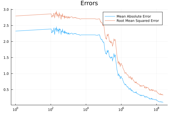
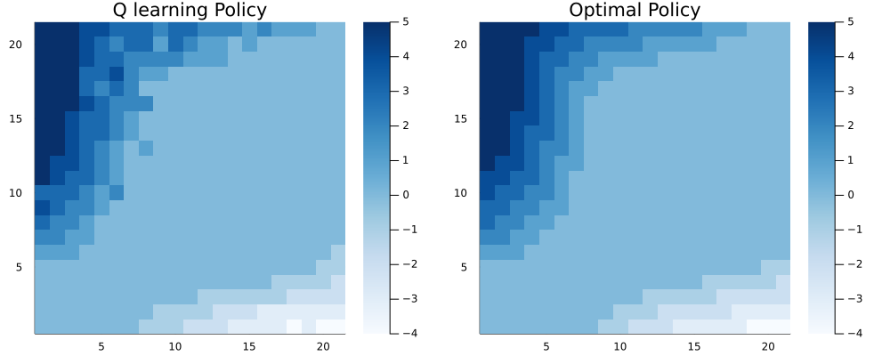
The final value of MAE is 0.107 and RMSE is 0.34. Here is the final step estimate for target policy next to the optimal one:

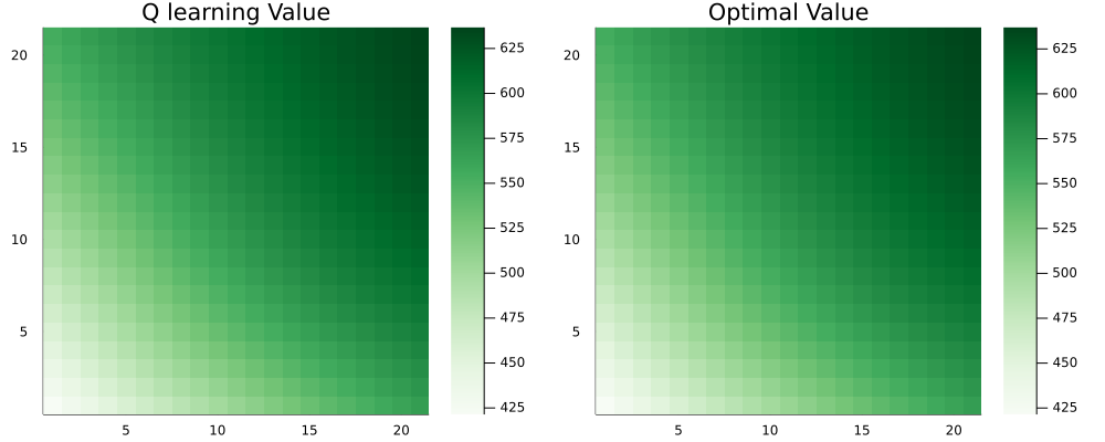
Under the target policy, the value differs from the optimal one by no more than 0.11% for any state:

The error plots indicate the “diminishing returns” - to get a little closer to the optimal policy takes ever more time steps. Tuning scheduling for $\alpha$ had the largest effect on the rate of the convergence.

Julia seems to be a great option for reinforcement learning due to its speed and Python-like convenience. Beyond tabular methods, when the environment model becomes the runtime bottleneck, Python will likely catch up thanks to high performance frameworks like Tensorflow or Pytorch. This is something I will explore in the future posts.