Flat Earth: a satellite image case
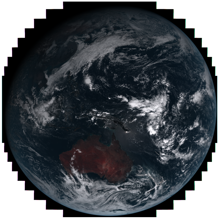 Eastern hemisphere on 7 December 2019
Summer of 2020 (Decemebr to February) in Australia became memorable for me for all the wrong reasons. Massive bushfires raged in the South Eastern part of the country for over a month. Satellite imaging opens a path towards early detection and monitoring of the fires in near real time. One such satellite, Himawari 8, takes an entire an image of the Eastern Hemisphere every 10 minutes with 17 optical channels, including red, green and blue. Historical observations from Himawari 8 are available for free from several sources, including AWS.
Machine Learning is a promising approach to these problems considering successes of its applications in computer vision. However a fixed convolution kernel in most popular architectures, when applied to raw images, would capture much larger area as we approach poles compared to equator. This occurs due to geostationary satellites like Himawari 8 observing the earth at a large distance (about 6 Earth’s radii), where different areas of the planet are visible at different tilt relative to the light captured by the onboard camera. One of the solutions to the problem consists of using a locally flat coordinate system for every sub-region of interest, which is something I would like to share below.
Locally-flat coordinates
Analysing geospatial data with Python can greately benefit from a rich ecosystem of tools, the first of which is pyproj. It enables to transform points defined in one coordinate system into another. Such transformation can be non-linear, as is the case with a flat satellite image, observed by onboard sensors, and spherical coordinates on the planet.
from pyproj import Transformer

longlat = "+proj=longlat +datum=WGS84"
hw8 = r.variables["geostationary"].proj4

projector = Transformer.from_proj(proj_from=longlat, proj_to=hw8, always_xy=True)
Two coordinate systems are defined here: longlat, a longitude-latitude coordinates, and hw8 coordinates in an image projection as it is seen by the satellite. The latter string looks like this
+proj=geos +lon_0=140.7 +h=35785863 +x_0=0 +y_0=0 +a=6378137 +b=6356752.3 +units=m +no_defs
As we can see, the origin of coordinates is at a point (140.7, 0). Next, a projector object, that trasforms from longlat coordinates to hw8 satellite coordinates is defined. It can be used to map a point on a globe onto the satellite image like so
projector.transform(150.5, -34.5)
which returns (866588, -3464526). By offsetting this value by minimum values of x, y and dividing over the resolution (1000), we get the pixel coordinates on the image. Taking a slice of 300 pixel both ways along both axis gets us a Southern East part of Australia that was heavily affected by fires on that day.
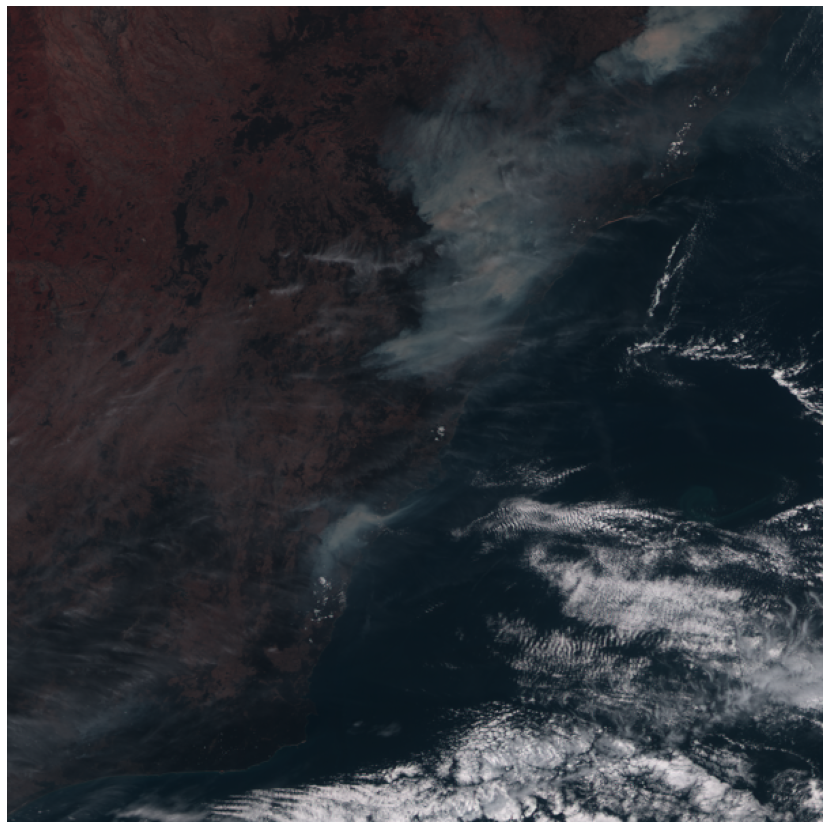
There is however a small problem - this part of the globe is tilted relative to the satellite position, so the image is distorted. This would create an above mentioned problem for an ML application.
A similar problem appears in General Relativity, where co-moving reference frame is locally flat and simplifies relevant equations. Constructing locally flat coordinates with a fixed resolution would place every observed point in the image on the same footing when it comes to convolutions.
One such coordinate system is an azimuthal equidistant projection which to a good approximation is locally flat near its center. Lets show this on the following example.
Firstly, define a projector object between longlat and new coordinate system aeqd
aeqd_local = "+proj=aeqd +lat_0=-34.5 +lon_0=150.5 +datum=WGS84"

projector = Transformer.from_proj(proj_from=aeqd_local, proj_to=longlat, always_xy=True)
and generate five random points inside the 600 by 600 km2 region
np.random.seed(42)

aeqd_points = list(zip(np.random.randint(W, E, 5), np.random.randint(S, N, 5)))

np.round(pairwise_distances(aeqd_points, aeqd_points, metric='euclidean'))
the resulting points are
[(-178042, -245114), (-168068, -162663), (65838, 221430), (-40822, -212502), (-189732, -124797)] and the pairwise distances, calculated with Euclidian metric between them are
array([[     0.,  83052., 526442., 141042., 120884.],
       [ 83052.,      0., 449710., 136658.,  43625.],
       [526442., 449710.,      0., 446848., 430336.],
       [141042., 136658., 446848.,      0., 172819.],
       [120884.,  43625., 430336., 172819.,      0.]])
Now, lets compare the distances between points calculated in longlat coordinates. The below code
from geopy.distance import geodesic

lonlat_points = list(projector.itransform(aeqd_points))
lonlat_points = [(pt[1], pt[0]) for pt in lonlat_points]

np.round(np.array([geodesic(pt1, pt2).m for pt1 in lonlat_points for pt2 in lonlat_points]).reshape(5, 5))
yields
array([[     0.,  83045., 526437., 141020., 120864.],
       [ 83045.,      0., 449704., 136633.,  43616.],
       [526437., 449704.,      0., 446848., 430325.],
       [141020., 136633., 446848.,      0., 172789.],
       [120864.,  43616., 430325., 172789.,      0.]])
As is evident from this simple example, the results produced by both methods are very close. Hence, this transform locally flattens the Earth.
In these new coordinates, this is what the region of interest looks like:
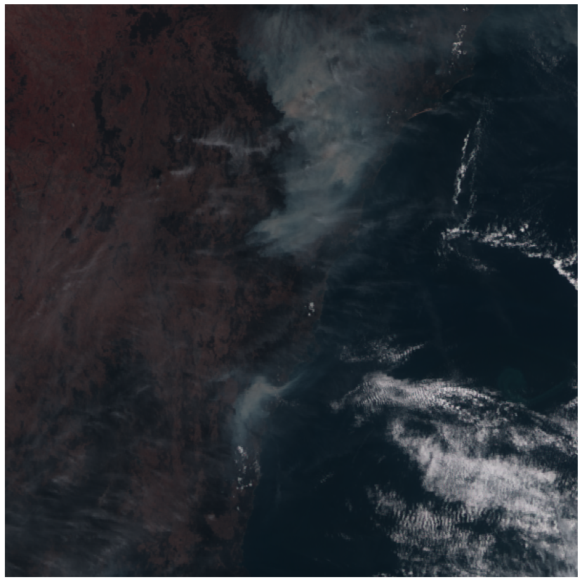
In the real applications, it desirable to get as much constrast between what you are looking for and the background. While fires are certainly visible to a naked eye, atmosphere and smoke hide it from the satellites view. This is where the near infra-red light (like band 7 of Himawari 8) comes in handy. Here is what it looks like in the locally flat coordinates (infrared on the right)
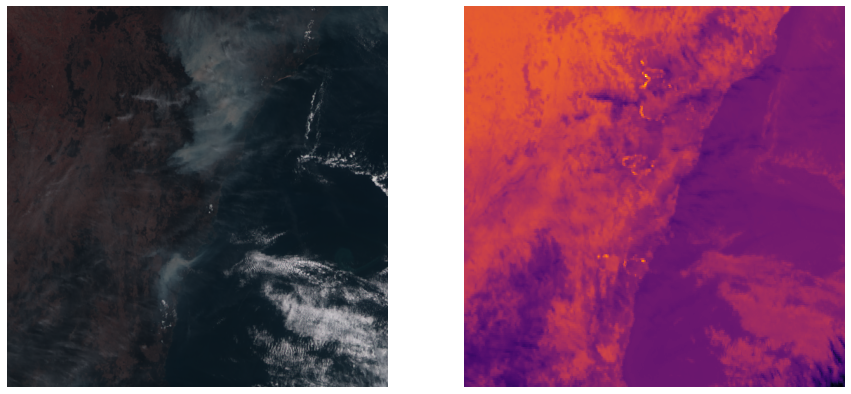
Bright contours clearly show the severity of fires that were raging in the region. Check this notebook for a full code.
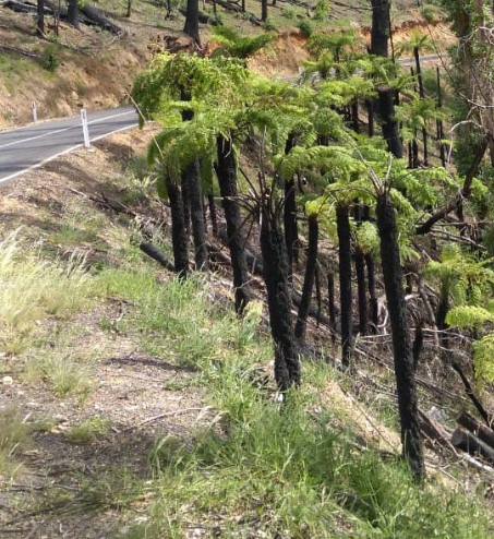
One thing that surprised me the most in Australian outback is that the local plant life has adapted to survive bushfires. Here is a picture of burned down ferns that I took in the mountains near Marrisvile that suffered a devastating bushfires in 2009