Hypothesis Testing with Z test
 Photo by Brett Jordan on Unsplash
Intoduction
By its nature, statistical tests give an answer to questions like:
- What is the probability of the observed difference be due to pure chance? (Q1)
For an actionalbe insight, a yes/no question is often preffered. In abstract terms, we seek to answer another question:
- Based on the observations, can we reject the null hypothesis $H_0$? (Q2)
where the null hypothesis $H_0$ refers to a statement that the treatment has no effect on the outcome. In terms of the business problem, the above question can sound something like
- Does the new website design improve the subscription rate by $1.5$% or more?
In this case, $H_0$ will be the statement that the new website design does not improve the subscription rate by at least $1.5$%
Before jumping into experiments, couple decisions need to be made. These are decisions about the tollerance we have to a random chance messing with the test and leading us to wrong conclusions. These have to be set before the start of the test to avoid bias in interpreting result. There are two types of error, so two thresholds to agree upon.
| Null Hypothesis Actually is | |||
|---|---|---|---|
| Decision | True | False | |
| Decision about Null Hypothesis | Don't Reject | Correct Decision (true positive) probability = $1 - \alpha$ | Type 2 Error (false negative) probability = $\beta$ |
| Reject | Type 1 Error (false positive) probability = $\alpha$ | Correct Decision (True negative) probability = $1 - \beta$ | |
The first one is the probability threshold $\alpha$ called sensitivity. Assume that $H_0$ was actually correct, treatment made no difference. If the estimated probability from Q1 is at or below $\alpha$, we incorrectly reject null hypothesis and conclude that the treatment made a difference. In particular, there is a less than $\alpha$ chance that the observed effect was purely due to random chance, which is reffered to as the type 1 Error. The latter means that we are willing to tollerate the potentially incorrect decision to reject $H_0$ if the probability of such a scenario is no more than $\alpha$.
The second one probability threshold $\beta$ considers the scenario when $H_0$ is actually incorrect, but the experiment indicates that it is not. The complementary probability, $1 - \beta$, is referred to as statistical power and describes a degree of certainty we want to have in been correct if we decide to reject $H_0$. In other words, statistical power gives us an expected fraction of correctly rejecting null hypothesis if we run many such experiments.
Example problem
To show how Z-test would work in practice, lets quantify the effect of treatment on the probability of a certain outcome. Consider a toy example:
“Does the new website design improve the subscription rate by at least $1.5$%?”
As an example, we seek to answer the above question. In the simplest case, we assume that
- For the experiment, customers are selected at random from a cohort that represents target audience
- Customers make decisions independent of each other
- Customer traffic is randomly split into two groups, A and B, depending on which version the website, new or old, they were presented with
- Each of two groups has sufficiently large (for Central Limit Theorem to work) number of customers
Experiment setup
Under these assumptions, the probability distribution for a number of subscriptions in each group is given by the binomial distribution with probabilities of a customer subscribing are $p_A$ and $p_B$ respectively. In addition, lets assume that for the old version of the website there is an estimate for the value of the subscription probability $p_A$, which is $8.5$%. From this point, we can use 5 steps 100 Statistical Test as a guide to setup the experiment
Step 1: Null Hypothesis
The null hypothesis states that $p_B - p_A < 0.015$, so that the new website design has less than the desired effect on the subscription probability.
In the language of mathematics, the null hypothesis $H_0$ states that $\mu = p_B - p_A = 0.015$.
Step 2: Sensitivity and Power
Next, we need to select values of sensitivity and power that we are comfortable with. Usually, $\alpha$ for sensitivity is selected to be between 1 and 10 percent, while for power $1 - \beta$ is of the order of at least 80 percent. For this example lets set
$$\alpha = 0.05$$ $$1 - \beta = 0.8$$
These values come from classical literature and aim to strike a balance between detecting the effect of treatment if it is present, while reducing the cost of collecting the data. For more detailed discussion check out p. 17 in Statistical Power Analysis for the Behavioral Sciences and p. 54, 55 in The Essential Guide to Effect Sizes.
Step 3: Test statistic
If the number of customers $N_A$ and $N_B$ is sufficiently large, we can invoke Central Limit Theorem to describe the probability distributions of the subscription number means in each group $$\overline x_A \sim N(p_A, \sigma_A)$$ $$\overline x_B \sim N(p_B, \sigma_B)$$
where $N(\mu, \sigma)$ is a normal distribution. For the test statistic $Z$, we can use the rule for a sum of normally distributed random variables
$$Z = \frac{\overline x_B - \overline x_A - \mu}{(\sigma_A + \sigma_B)^{1/2}} \sim N(0, 1)$$
If the p-value for the test statistic is at or below $\alpha = 0.05$, we must reject $H_0$ and accept an alternative hypothesis $H_1$ that version B of the website does improve the subscription rate by $1.5$ % or more than the current version A.
Step 4: Confidence Interval for test statistic
Based on test statistic $Z$ and sensitivity $\alpha$, select critical region. It is evident from the null hypothesis that we need to use a one-tail region $Z < Z_c$ only. Since $Z$ is described by a normal probability distribution function (pdf),
critical value is $Z_c \approx 1.64$ for $\alpha = 0.05$
Corresponding cumulative distribution function for this critical value $Z_c$ covers $100\times(1 - \alpha) = 95$ % interval. Should the value of test statistic fall inside the interval $(-\infty, Z_c)$, we accept null hypothesis, otherwise we accept an alternative hypothesis.
Step 5: Effect Size and Sample Size
Finally, lets estimate a minimal sample size required to achieve desired statistical power. In addition to sensitivity and power, effect size needs to be evaluated, which requires a priori information and / or assumptions. For equal number customers in both groups with the assumption that this number is sufficiently large (so that the sampling distribution is well approximated a normal one), Cohen’s D can be used to approximate effect size
$$D = \frac{|p_B - p_A|}{\sigma}$$
where $\sigma^2 = s_A^2 + s_B^2$ and $s_{A(B)} = \sqrt{p_{A(B)}(1 - p_{A(B)})}$. Such estimate would require an assumption that a good estimate for $p_B$ is available, which is likely unrealistic. Nevertheless, assume that
A good estimate for $p_B$ is $11$%
Substituting the parameters, we find $D = 0.0239$.
Estimating required number of test participants
With all pieces of the puzzle in place, we can proceed to estimating sample size from effect size, sensitivity and power. Python statsmodel package comes handy for this task
from statsmodels.stats.power import NormalIndPower

ALPHA = 0.05
BETA = 0.2

PowerAnalysis = NormalIndPower()

N_total = PowerAnalysis.solve_power(effect_size=D, alpha=ALPHA, power=1 - BETA, alternative="larger", ratio=1)
The calcalation returns $21723$ for a minimal total number of customers in both groups, or $N_{A(B)} = 10862$ in each group.
Under the hood, above code involves numerically solving this equation for $N_{A(B)}$
$$\beta = \Phi(Z_c - D\times\sqrt{N_{A(B)}})$$
where function $\Phi$ is a probit function, an inverse of cumulative distribution function (CDF) for the normal didistribution. With power $1 - \beta = 0.8$ we can verify this by substituting the result into a CDF for the normal distribution, which should be $\beta = 0.2$ or less:
from scipy.stats import norm

Zc = 1.64

norm.cdf(Zc - D*np.sqrt(N_total/2))
returns $0.199$.
Code for Experiments
Here is the notebook with the whole code. Each experiment consists of simulating the observed data and running the Z-test for this data.
from statsmodels.stats.weightstats import ztest
import numpy as np

def run_ztest(p0, p1, N_samples, value):
    # generate data
    data_0 = np.random.binomial(1, p0, N_samples)
    data_1 = np.random.binomial(1, p1, N_samples)

    # run Z-test
    result = ztest(data_1, data_0, alternative="larger", value=value)

    return result
The above code generates two sets of data, for both groups $p_A$ and $p_B$, which simulates the actual observation. Next, function ztest returns two values, test statistic $Z$ and p-value, the probability that data sets come from the same distribution, which corresponds to null hypothesis. Parameter value is set to the threshold value of the effect $0.015$ ($1.5$ %). Parameters p0 and p1 are the true, unknown values for probabilities of subscription.
Experiments
True subscription rate due to new website design either exceed or is below the threshold. Consider the former case when it exceeds the threshold and null hypothesis has to be rejected. The analysis is the same for the latter case. In the considered case lets focus on the Type II Error, when the test shows that the new website design does not achive the goal.
There are three possible scenarios for the true value of subscription probability in group B compared to the estimate $p_B = 0.11$ that we obtained:
- $p_{true} \approx p_B$
- $p_{true} < p_B$
- $p_{true} > p_B$
In each of these scenarios the chances of making correct decision whenever or not to reject null hypothesis. Lets consider each of these possibilities.
Actual subscription probability is $11$ % due to the new website design
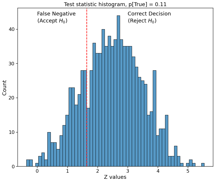
Good estimate for $p_B$ allows to accurately estimate the effect size, and consequently the number of participants required to achive the target statistic power of $80$ %. Running 1000 identical tests, correct decision will be made in $77.9$ %.
Actual subscription probability is $10.5$ % due to new website version
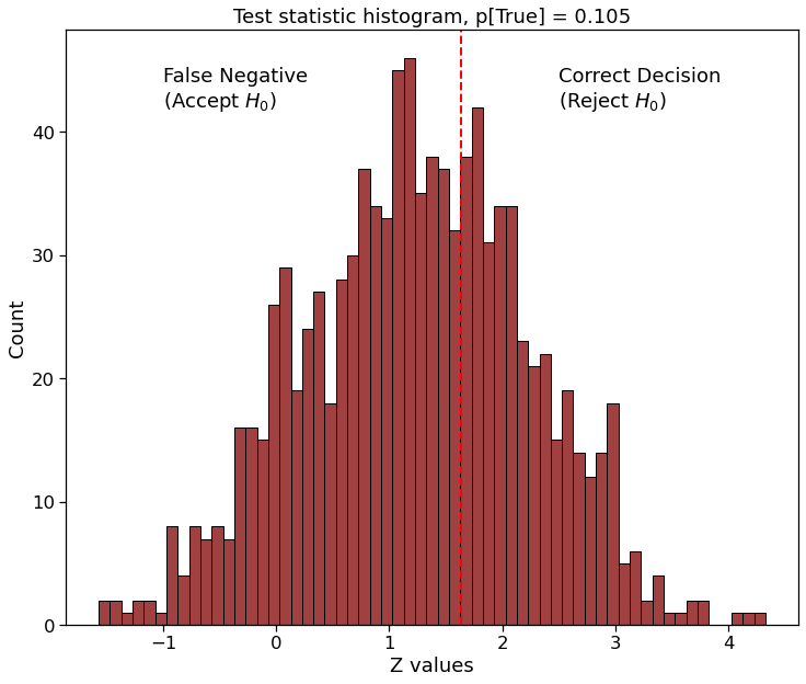
Estimate for $p_B$ was too optimistic, resulting in overly high effect size. Running 1000 identical tests, correct decision will be made in $35.8$ %. However, the subscription probability exceeds the target of $1.5$ % improvement. To get a good confidence in the test, more samples are needed.
Actual subscription probability is $11.3$ % due to new website version
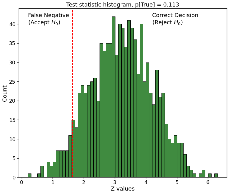
Estimate for $p_B$ was too pesimistic, resulting in overly conservative effect size. On the good side, running 1000 identical tests, correct decision will be made in $93.6$ %.
Even though in all of the above cases the new website design achieved the goal, out chance of picking it with Z-test was dramatically different. One way to address this is to be more conservative when estimating effect size, but that might be incure costs in practice. Another is to explore different test setups, which is my future quest.