Optimizing Jack's Car Rental

While enjoying an excellent book, titled “Reinforecement Learning” by Richard Sutton and Andrew Barto, a toy problem on page 81 has drawn my attention. It is titled “Jack’s Car Rental” and goes as follows:

Jack manages two locations for a nationwide car rental company. Each day, some number of customers arrive at each location to rent cars. If Jack has a car available, he rents it out and is credited 10 by the national company. If he is out of cars at that location, then the business is lost. Cars become available for renting the day after they are returned. To help ensure that cars are available where they are needed, Jack can move them between the two locations overnight, at a cost of 2 per car moved. We assume that the number of cars requested and returned at each location are Poisson random variables, meaning that the probability that the number $n$ is $\lambda^ne^{-\lambda}/n!$ , where $\lambda$ is the expected number. Suppose $\lambda$ is 3 and 4 for rental requests at the first and second locations and 3 and 2 for returns. To simplify the problem slightly, we assume that there can be no more than 20 cars at each location (any additional cars are returned to the nationwide company, and thus disappear from the problem) and a maximum of five cars can be moved from one location to the other in one night. We take the discount rate to be $\gamma$ = 0.9 and formulate this as a continuing finite MDP, where the time steps are days, the state is the number of cars at each location at the end of the day, and the actions are the net numbers of cars moved between the two locations overnight.

The main objective of the problem is to determine an optimal policy - the number of cars to be transferred from location 2 to location 1 (or vise versa) in order to maximise the expected profit. Below I would like to share my solution.

Lets start by introducing some mathematical notations to describe Jack’s daily routine:

• At the end of the day Jack counts $N_1$ cars at the first location (P1) and $N_2$ cars at the second (P2), so the state is $s = (N_1, N_2)$.
• Next, Jack decides to take an action and move $a$ cars from P1 to P2, which gets him to $(N_1{''} = N_1-a, N_2{''}=N_2+a)$ car arrangement at the start of the next day.
• At the end of next day at each location $X_i$ ($i = 1, 2$) cars were rented out and $Y_i$ were returned. The new state at the end of next day is $s' = (N_1{'}= N_1{''}-X_1+Y_1, N_2{'}=N_2{''}-X_1+Y_1)$

The reward (profit) at the end of next day is

$$r = R_x\sum_{i=1, 2}X_i + R_a|a|,$$

where $R_x = 10$ and $R_a = -2$. According to the problem condition, each location does not fit more than $N_{max} = 20$ cars, so that $N_i, N_i{'}, N_i{''} \in [0, 20]$ and at most 5 cars can be moved so that $a \in [-5, 5]$. A negative value of $a$ indicates a transfer of cars in the opposite direction, from P1 to P2.

Policy and Value

For the sake of consistency, lets briefly review key quantities we are looking to find, policy and value. Policy determines which action $a$ an acting agent, Jack in this case, should take in response of finding himself in the state $s = (N_1, N_2)$. In mathematical terms, the policy $\pi = \pi(a | s)$ is a conditional probability, hence a stochastic function of $a$ and $s$ that an agent seeks to determine. In our problem however, it is a purely determininstic function

$$\pi(a | s) = \pi(s) = \mathbb{1}_{a=\pi(s)}.$$

Intuitively it is clear that the agent seeks to find the optimal policy that maximises the reward. But which reward is it? An immideate reward for the next day, or a comdined reward for the next 10 years? Following a “long-term greedy” principle we seek to maximise the total reward for all days that follow $\sum_{t=1}^{\infty}R_t$. However, mathematically such series can and almost always do diverge. Introducing an artificial factor $\gamma \in (0, 1)$ into $G = \sum_{t=1}^{\infty}\gamma^t R_t$ removes this problem for most realistic future rewards. In literature this trick is referred to as gamma discounting and yield the **value** function

$$\upsilon(s) = E_{\pi}(G | s).$$

The value that corresponds to an optimal policy satisfies Bellman optimality equation (see page 63 in “Reinforcement Learning” book). It is a non-linear equation, which can be solved using an iterative algorithm. At every iteration both value and policy approach their optima.

Evaluate and Impove

Consider the iterative algorithm for optimising the car transfer policy on page 80. The algorithm evaluates the value function

$$\upsilon(s) = \sum_{r, s{'}} p(s{'}, r | s, a = \pi(s)) \left(r + \gamma\upsilon(s')\right)$$

and then uses it to improve the policy

$$\pi(s) = \arg\max_a \sum_{r, s{'}} p(s{'}, r | s, a) \left(r + \gamma\upsilon(s{'})\right)$$

Here $p(s{'}, r | s, a)$ describes the external environment and gives a probability of finding oneself in the state $s'$ with a reward $r$ if an action $a$ was taken in the state $s$.

Since there are 11 different car moving options (up to 5 cars between both parkings), both states $s'$ and $s$ have dimensions of $21^2$, the tensor of conditional probabilities $p(s', r | s, a)$ has at least $11\times21^4 = 2139291$ values. The actual number it is larger thanks to the reward dimension $r$ that we did not count. If Jack manages three rather than two carparks and can transfer up to 5 cars between each two, the probability tensor has over 114 trillion elements (not counting the reward dimension).

Looking at $p(s', r | s, a)$ I have experienced a dejavu, as those kind of dimensionality problems are quite routine in theoretical atomic physics. In short, it pays to have a closer look and do some math rather than head-on coding multiple nested loops.

Firstly, notice that the right hand sides of both equations are mostly the same, and can be simplified:

$$\sum_{r, s'} p(s', r | s, a) \left(r + \gamma\upsilon(s{'})\right) = r(s, a) + \gamma\sum_{s{'}}p(s{'} | s, a)\upsilon(s{'}),$$

where $r(s, a) = \sum_{r, s{'}} p(s{'}, r | s, a) r$ is the expected reward in a state $s=(N_1, N_2)$ if $a$ cars are transferred from P2 to P1 and $p(s{'} | s, a) = \sum_{r}p(s{'}, r | s, a)$ is the probability of transitioning to a state $s{'} = (N_1{'}, N_2{'})$ the next day from from a state $(N_1, N_2)$ and $a$ cars getting transferred. This little mathematical juggling replaced a massive 6D tensor $p(s{'}, r | s, a)$ with a smaller 3D $r(s, a)$ and 5D $p(s{'} | s, a)$ tensors, that can be further simplified and efficiently calculated.

Expected reward and state transition probability

Expected reward tensor $r(s, a)$ is a 3D tensor and can be evaluated once at the start. Since after the cars are transferred, the reward from each car park is statistically independend, for the total reward we can write

$$\begin{array}{c} r((N_1, N_2), a) = R_x\sum_{X_1 = 0}^{N_1{''}}X_1p(X_1|\lambda_1, N_1{''}) + \\\
R_x\sum_{X_2 = 0}^{N_2{''}}X_2p(X_2|\lambda_2, N_2{''}) - R_a|a|,\end{array}$$

where

$$p(X|\lambda, N) = \begin{cases} p(X | \lambda) & \quad X < N \\\ \sum_{Z=N}^{\infty} p(Z | \lambda) & \quad X = N \end{cases}$$

is the probability of $X$ cars rented out from a location that had $N$ cars at the start of a day. The probability of demand reaching $X$ cars at a particular location with a mean demand $\lambda$ follows the Poisson distribution.

Next, lets further simplify the transition probability. Like first two terms in the above equation for the expected reward, the transition probability depends on $N_1, N_2, a$ only as

$$\begin{array}{c}p((N_1{'}, N_2{'}) | (N_1, N_2), a) = p((N_1{'}, N_2{'}) | (N_1{''}, N_2{''})) = \\\ p(N_1{'} | N_1{''})p(N_1{'}|N_1{''}).\end{array}$$

For $i$-th location, the probability of starting the day with $N_i{''}$ cars and ending it with $N_1{'}$ can be evaluated as

$$\begin{array}{c}p(N_i{'}|N_i{''}) = \sum_{X_i = 0}^{N_i{''}}p(X_i|\lambda_i, N_i{''})\times \\\ p(Y_i=N_i{'}-N_i{''}+X_i|\mu_i, N_{max} - N_i{''}+X_i),\end{array}$$

where $\mu_1 = 3$ and $\mu_2=2$ are average numbers of returned cars at each location. If the $Y = N{'}-N{''}+X < 0$ in the above exression, then the probability $p(Y|\mu, N)$ should be set to zero as the number of returned cars cannot be negative.

Therefore, the 5D tensor of transition probabilities $p(s{'} | s, a)$ can be represented as a product of two 2D conditional probability tensors $p(N_i{'}|N_i{''})$.

Implementation

The maths above enables to write both expected reward and transition probability in a compact form

$$\begin{array}{c} r(s, a) = R{''}(N_1{''}, N_2{''}) + R_a|a| \\\ p(s{'} | s, a) = P^{(1)}(N_1{'}, N_1{''})P^{(2)}(N_2{'}, N_2{''})\end{array}$$

This enables to write the right-hand-size of Bellmans equation as

$$\sum_{r, s'} p(s', r | s, a) \left(r + \gamma\upsilon(s{'})\right) = RHS(N_1{''}, N_2{''}) + R_a|a|$$

where matrix $RHS = R{''} + P^{(1)T}VP^{(2)}$ can be efficiently calculated for both evaluation and improvement steps. A complete source code can be found on my Github. Lets go through it step by step.

Here is a list of paramets given by the problem

# Maximum number of cars at each location
N_MAX_CARS = 20

# Maximum number of cars that can be transferred by Jack
A_MAX = 5 

# Mean number of cars of rented out at each location
LAMBDA = [3, 4]

# Mean number of cars returned to each location
MU = [3, 2]

# Dicount rate
GAMMA = 0.9

# Reward for each car Jack decides to transfer
R_A = -2

# Reward for each car that gets rented
R_X = 10

The right-hand-side matrix $RHS$, denoted as RHS_N__ in the code, is calculated as

RHS_N__ = R_N__ + GAMMA * P1.T.dot(value).dot(P2)

where R_N__ is $R''(N_1{''}, N_2{''})$, P1 ($P^{(1)}$) and P2 ($P^{(2)}$) are the transition matrixes for individual locations. For the sake of time, I will not present the calculation of these matrixes. They are a straightforward implementation of the above equation, and can be found in the notebook.

The Value Iteration code looks like this

def IterValue(value, policy, toll=1e-3, max_iter=100):
    """
    Iterate value until maximum difference between successive
    iteration is under a tollerance threshold.
    """
    delta = 1
    it = 0
    
    while delta > toll and it < max_iter:
        it += 1

        value_new = np.zeros(value.shape)
        # Combine all matrixes in (N_, N__) on the right-hand-side of
        # the Bellmans Equation
        RHS_N__ = R_N__ + GAMMA * P1.T.dot(value).dot(P2)

        for N1 in range(value.shape[0]):
            for N2 in range(value.shape[1]):
                a = policy[N1, N2]
                N1__ = N1 - a
                N2__ = N2 + a
                
                if N1__ < 0 or N1__ > N_MAX_CARS: continue
                if N2__ < 0 or N2__ > N_MAX_CARS: continue

                value_new[N1, N2] = RHS_N__[N1__, N2__] + R_A * abs(a)

        delta = np.max(np.abs(value - value_new))
        value = value_new
    
    if (it < max_iter): print(f"Value iteration converged in {it}
    iterations.")
    else: print(f"Too many iteration. Final delta --- {delta}.")
        
    return value

Using Value and Policy, initialized with zeros it can be ran like so

Value = np.zeros((N_MAX_CARS + 1, N_MAX_CARS + 1))
Policy = np.zeros((N_MAX_CARS + 1, N_MAX_CARS + 1), dtype=np.int16)

Value = IterValue(Value, Policy)

and takes about a 0.25 seconds to run a 100 iterations on my desktop. Next, lets consider the Policy improvement code

def ImrovePolicy(value, policy):
    """
    Apply policy improvement part of the algorithm.
    """
    # Combine all matrixes in (N1__, N2__) on the right-hand-side of
    # the Bellmans Equation
    RHS_N__ = R_N__ + GAMMA * P1.T.dot(value).dot(P2)

    for N1 in range(value.shape[0]):
        for N2 in range(value.shape[1]):
            v_max = -np.inf
            a_max = 0
            for a in range(-A_MAX, A_MAX + 1):
                N1__ = N1 - a
                N2__ = N2 + a
                              
                if N1__ < 0 or N1__ > N_MAX_CARS: continue
                if N2__ < 0 or N2__ > N_MAX_CARS: continue
                
                v_candidate = RHS_N__[N1__, N2__] + R_A * abs(a)
                
                if v_candidate > v_max:
                    v_max = v_candidate
                    a_max = a
            
            policy[N1, N2] = a_max

    return policy

Running both stages sequentially gives a single iteration of the Evaluate and Improve algorithm:

Value = IterValue(Value, Policy, toll=1e-3)
Policy = ImrovePolicy(Value, Policy)

Results

The algorithm converges in 5 iterations. The result for Policy looks like this

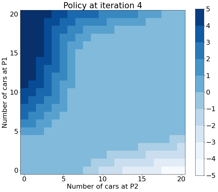
Jack can use the above map much like a chart of Texas Holdem starting hands. The cell that corresponds to the number of cars at the end of the day in both location gives a number of cars to be transferred from P1 to P2 that gives an optimal expected Value.

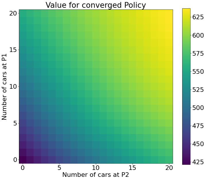
Under this optimal Policy the Value that Jack should expect to get looks like this: